1.
choropleth party
2.
R for Global Wind Wave / Wave Swell Forecasting
As a follow up to using freely available existing climate datasets,here's one that might be of interest to those surfers and sailorsout there. It is similar approach to that used for the temperature forecasting so go read that post first, it will help.
The free information from the U.S. NOAA/National Weather Service's National Centers for Environmental Prediction, in particular its Environmental Modeling Center and its WaveWatch dataset. It is stored as a GRIB2 files and this needs to be pre-processed using wgrib2 (available on MacPorts) to the netcdfformat. This stage is similar to the previous post.
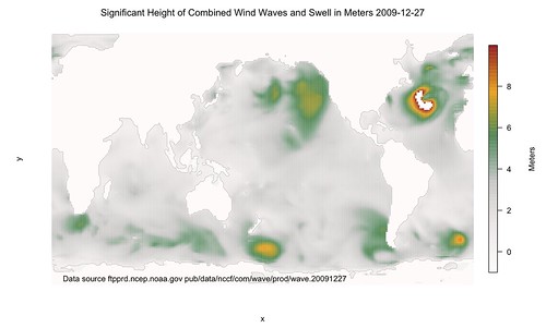
There were a few little glitches with this dataset that are immediately visible and the fact there is a big white patch in the Atlantic is due to the maximum height being stored as 9.999e+20. This normally won't be a problem but unfortunately the data also stores dry land with this value. A workaround would be to know or compute longitudes and latitude such that we could tell if a given position was over land or over sea prior to processing it. Unfortunately as this is a bit of a quick and dirty hack, I didn't have the time so here is the basic approach warts and all.
http://www.nco.ncep.noaa.gov/pmb/products/wave/nww3.t00z.grib.grib2.shtml
# Data was from ftp ftpprd.ncep.noaa.gov dir: /pub/data/nccf/com/wave/prod/wave.20091227
# wgrib2 was installed using macports
# /opt/local/bin/wgrib2 -s nww3.t00z.grib.grib2 | grep "HTSGW:surface:an" | /opt/local/bin/wgrib2 -i nww3.t00z.grib.grib2 -netcdf WAVE.nc
library(ncdf)
waveFrac <- open.ncdf("WAVE.nc")
wave <- get.var.ncdf(waveFrac, "HTSGW_surface")
# Dirty hack to fix input model, look for another better solution
wave[wave>9.99999]<- -1
x <- get.var.ncdf(waveFrac, "longitude")
y <- get.var.ncdf(waveFrac, "latitude")
library(fields)
rgb.palette <- colorRampPalette(c("snow1","snow2","snow3","seagreen","orange","firebrick"), space = "rgb")
image.plot(x,y,wave,col=rgb.palette(255),axes=F,main=as.expression(paste("Significant Height of Combined Wind Waves and Swell in Meters 2009-12-27", sep="")),legend.lab="Meters")
# Add a rough outline for islands, countries, and continents
contour(x,y,wave,add=TRUE,lwd=0.25,levels=0.2,drawlabels=FALSE,col="grey30")
# Add the source of the file and ftp location
text(130,-75,"Data source ftpprd.ncep.noaa.govpub/data/nccf/com/wave/prod/wave.20091227")
# ftp.ncep.noaa.gov pub/data/nccf/com/gfs/prod/gfs.2009121700
# See http://www.nco.ncep.noaa.gov/pmb/products/gfs/gfs.t00z.sfluxgrbf00.grib2.shtml
# eoin-brazils-macbook-pro:~ eoinbrazil$ cp gfs.t00z.sfluxgrbf03.grib2 temp2.grb
# wgrib2 was installed using macports
# /opt/local/bin/wgrib2 -s temp2.grb | grep ":LAND:" | /opt/local/bin/wgrib2 -i temp2.grb -netcdf LAND2.nc
# /opt/local/bin/wgrib2 -s temp2.grb | grep ":TMP:2" | /opt/local/bin/wgrib2 -i temp2.grb -netcdf TEMP2.nc
library(ncdf)
landFrac2 <- open.ncdf("LAND2.nc")
land2 <- get.var.ncdf(landFrac2, "LAND_surface")
x <- get.var.ncdf(landFrac2, "longitude")
y <- get.var.ncdf(landFrac2, "latitude")
library(fields)
rgb.palette <- colorRampPalette(c("snow1","snow2","snow3","seagreen","orange","firebrick"), space = "rgb")
tempFrac2 <- open.ncdf("TEMP2.nc")
temp2 <- get.var.ncdf(tempFrac2, "TMP_2maboveground")
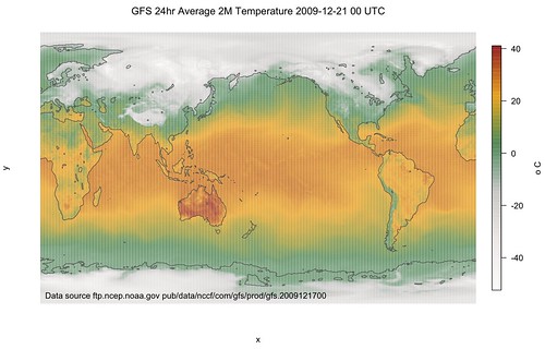
newtemp2 <- temp2-273.15 # Convert the kelvin records to celsius
image.plot(x,y,newtemp2,col=rgb.palette(200),axes=F,main=as.expression(paste("GFS 24hr Average 2M Temperature 2009-12-21 00 UTC",sep="")),legend.lab="o C")
contour(x,y,land2,add=TRUE,lwd=1,levels=0.99,drawlabels=FALSE,col="grey30") #add land outline
text(120,-85,"Data source ftp.ncep.noaa.gov pub/data/nccf/com/gfs/prod/gfs.2009121700")

How the map was made
GFS forecasts are in a format called GRIB2. According to Wikipedia,
“GRIB (GRIdded Binary) is a mathematically concise data format commonly used in meteorology to store historical and forecast weather data.” GRIB files contain physical fields such as temperature, humidity etc defined on a spatial grid, as well as boundary conditions such as vegetation type and elevation. The data might be assimilated from observations, or output from a forecast model.
The first step is to translate the GRIB into a raster format such as
netcdf which can be read in
R. For example, the GRIB2 file
gfs.2009121700/gfs.t00z.sfluxgrbf03.grib2 contains the 3-hr forecast surface data on 17 Dec 2009 produced at 00 UTC (midnight universal time). An inventory of the data contained in this file can be seen
here. Download this forecast as
temp.grb
loc=file.path("ftp://ftp.ncep.noaa.gov/pub/data/nccf/com/gfs/prod/gfs.2009121700/gfs.t00z.sfluxgrbf03.grib2")
download.file(loc,"temp.grb",mode="wb")
To read
temp.grb a utility called
wgrib2 needs to be installed on your system. Then data such as land fraction can extracted into a netcdf file
LAND.nc using the
R shell command
shell("wgrib2 -s temp03.grb | grep :LAND: | wgrib2 -i temp00.grb -netcdf LAND.nc",intern=T)
The ncdf package can now be used to read the contents of LAND.nc.
library(ncdf)
landFrac <-open.ncdf("LAND.nc")
land <- get.var.ncdf(landFrac,"LAND_surface")
x <- get.var.ncdf(landFrac,"longitude")
y <- get.var.ncdf(landFrac,"latitude")
The 1152×576 matrix land takes values 1 for land and 0 for water (sea-ice is 1). x and y are the longitude and latitude of the non-uniform GFS grid.
2m temperature data can be read in the same way. The average of the first 8 forecasts was called t2m.mean and plotted using image.plot() from the fields package:
library(fields)
rgb.palette <- colorRampPalette(c("snow1","snow2","snow3","seagreen","orange","firebrick"), space = "rgb")#colors
image.plot(x,y,t2m.mean,col=rgb.palette(200),axes=F,main=as.expression(paste("GFS 24hr Average 2M Temperature",day,"00 UTC",sep="")),axes=F,legend.lab="o C")
contour(x,y,land,add=TRUE,lwd=1,levels=0.99,drawlabels=FALSE,col="grey30") #add land outline

没有评论:
发表评论